The Uncountable platform allows you to create models based on past data and use them for making predictions. With a decent model, you might be able to predict the properties of formulations before conducting the experiments or even without necessarily conducting them in the lab.
You have a couple of handy options when it comes to making a predictive model: you can select which formulations to include or exclude, you can select which inputs to be used as predictors or non predictors, you can select which outputs to be modeled, you can select different types of models (linear, non-linear …) to work with, you can also view model surface using different visualization tools on the platform: e.g. model plots, interaction explorer.
One important concept to note before we start: Unlike Suggest Experiments with AI (which is another popular option under the Design tab), this method does not evolve an objective function. Thus, Analyze Experiments with AI allows you to make predictions with new formulations, however it will not suggest to you which experiments you should run next.
This article can walk you through various ways/address common questions in which you can set up, train, and model experiments.
Step 1. Select a Training Data Set

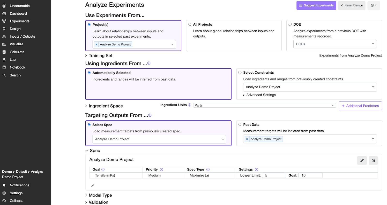
You can get to Analyze Experiments with AI page by clicking on the Design tab, and then select “Analyze Experiments with AI”
1.1 Use Experiments From
There are three options for you to choose:
Project(s) – the current project
All Projects – all of the projects in the current material family
DOE – only pick this if you have performed a set of DOE through the Uncountable platform
For most scenarios, it is advisable to use the analyze tool to select only data from within the project (the default option), so you can have a consistent set of ingredients and process parameters as input features for your model, and the correct measurements of interest to be modeled.
However, we have provided the option to incorporate data from outside the project, in the material family as a whole, to build a predictive model. Please select the option “All Projects” to use this wider data source, and only do so if you have access to, and are familiar with, the data outside the current project. This can sometimes be a good choice since training a model on more data would make it generalize better. You can refer to this article about how much data is needed to have good predictions. – link to https://www.support.uncountable.com/knowledge-base/troubleshooting-models-and-faqs/#31-how-much-data-is-needed-to-have-good-predictions
If you have performed a set of DOE experiments through the Uncountable platform or with external DOE tools and only want to include experiments from that particular DOE, you may pick the third option listed above. Using the default settings for selecting from the current project would already include the past DOE’s data.

1.2 Training Set Refinement
Having a good training set is important to build a good predictive model with useful accuracy. The Uncountable model training procedure can automatically exclude some outlier experiments, but you can also help build a good training set by excluding these experiments from the training set:
- Experiments that are far outliers in terms of the types or amounts of ingredients used.
- Experiments that have incomplete input data, particularly for important process parameters.
- Experiments that, in your expert assessment, have unreliably recorded measurement data.
Step 2. Select input features – Use Ingredients From
Input features are the independent variables of your project, which a model will use to build a predictive model. They are what you are using to predict.
You have 2 options below:
You may elect to use the Uncountable platform’s automatic selection of input features (via staying with the “Automatically Selected” option which is checked by default), which will automatically choose the most common input features in your data set.
You may also create constraints by yourself and use it for training a model. When setting up project constraints, it is important not to select too many input features to build your model. A model with more input features than data points is not meaningfully predictive. It is also important not to omit common and important input features from your model, since doing so is telling the model to ignore these input features. You can refer to this article about setting up proper constraints. – link to https://www.support.uncountable.com/knowledge-base/troubleshooting-models-and-faqs/
Step 3. Select outputs to predict – Targeting outputs from
Under this section, you will need to select measurements of interest on the Uncountable platform. They are what you are predicting.
Uncountable models are informed about what measurements are of interest through a Spec. You may inform the model about which measurements are important beforehand by constructing a Spec, including setting the right condition parameters for each output.
Since we are not producing recommended experiments, and are only building a model for analysis, it is not necessary to set the priorities or threshold for a Spec meant for analyzing data. The Uncountable platform creates a model for each measurement of interest, and the priorities and goals do not affect how the models are built.
You may also elect to use the Uncountable platform’s automatic selection of outputs as detected from past data. (via checking the “Past Data” option)

Step 4. Select the Model Type
The Uncountable Platform is built atop Uncountable’s models, which are based on a Matérn-kernel Gaussian Process (GP). Much of the platform’s functionality, especially for suggesting experiments with AI, uses the GP.
However, for the sake of comparative analytics, you are also able to train a variety of different types of models to analyze alongside the Uncountable GP model. These models can also be used for predictive purposes, and can be visualized using surface visualizations. The different models currently available on the Uncountable platform are:
- Ordinary least squares linear regression
- Ridge regression
- Gradient-boosted decision trees with XGBoost
- Random forest
- Neural network
For each model, there are certain hyperparameters the users can tune. For example, for GP, users can choose different initial length scale, weight regularization, the types of commonly used kernel functions. For random forest, users can choose the number of estimators, maximum tree depth, the criterion function …
It is likely that the model most suited to small and noisy data sets, which is the majority of experimental data sets, would be the GP.– link to https://www.support.uncountable.com/knowledge-base/troubleshooting-models-and-faqs/#1-how-does-uncountable-build-their-models
You can train any variety of these models alongside each other to compare which model is most suited to your data if you wish. If you pick more than one model to train, later in Step 6, each model will have its own training accuracy table displayed on the page.
Step 5. Validation
By default, we use leave-one-out validation. For a dataset with n number of data points. Everytime, we mask off one data point and use the rest n-1 data points to predict on that one. We proceed with this process n times until all data points have been predicted. This leave-one-out cross validation method provides a much less biased measure of mean squared error compared to using a single test set.
We also provide k-fold cross validation. The platform will randomly divide the dataset into K groups of approximately equal size. Then use each group as a test set for a model trained on the remaining (K-1) groups. When K gets large, training with cross validation will take more time. When k-fold cross validation is selected, in Step 6, the training accuracy table will be broken into k+1 subsection. One for the overall model performance (assuming leave-one-out was used), k for the model performance for each fold.
At this stage, you can click the “Train Model” button which is on the left corner of the page to start model training. It usually takes 1-10 minutes to train a model.

Step 6. Interpreting the Model’s Fit
The Training Accuracy table informs you about the performance of the model.
For each output, the following is displayed under the training accuracy section:
- RMSE – This is the model’s predictive error, and the lower the RMSE, the more accurate the model’s predictions are. This RMSE is calculated from the leave-one-out cross-validation procedure mentioned above. It will differ if you pick the k-fold cross validation.
- r² Score – This is the Coefficient of Determination, and the higher it is and closer to 1, the better the explanatory power of your model. It is one way of assessing how much of the variance and the range of the output of your data set can be explained by the model created.
- Explained Error – The Explained Error compares the magnitude of the RMSE with the magnitude of the standard deviation of your data. Since the RMSE is an absolute measure, the magnitude of which can differ from output to output, normalizing based on the standard deviation helps you to compare between different outputs. The higher the Explained Error, and closer to 100%, the more accurate the model’s predictions are.
- Scatter Plot of Predicted vs. Actual: In many ways one of the most intuitive and informative measures of predictive quality. The Uncountable platform analyzes all current data points, and uses them to predict each other data points in the plot. We want the model’s predictions to be close to the actual values of the experiments in the training data set, i.e. the points should lie close to the diagonal gray line on the graph. In the scatter plot view, look out for the following:
- Outliers, if one or two points have predictions that are very different from the actual values, more so than all other data points. Are the measurements from these experiments reliable? If not you should remove them from the training data set or tag them as outliers on the dashboard or enter measurement page.

- “Vertical lines” like those in the following figure:
This indicates that the model is making the same prediction for several points that have different actual measurements. The three most common reasons for this are 1) blank process parameter data, since those are interpreted by the model to be “0”, remove data points that have incomplete process parameters or remove these process parameters from the model features, 2) missing important input features, make sure that all important ingredients and process parameters are part of your Constraint used to create the model, 3) hidden subgroups of the data, check to see that the experiments you are putting together are not from different groups or experimental conditions that should not be mixed together.
Step 7. Analysis and Visualize Methodologies with the Uncountable Platform

7.1 Effect Sizes Table and Correlations
The Effect Sizes Table is a simplification of the model’s view of the underlying data. Most models are non-linear and non-straightforward, but the effect size boils down the general trend of an ingredient or parameter’s effect on a particular measurement into a single number. By default, the values in the table represent the magnitude of increase or decrease in the measurement value based on one standard deviation increase in the input value. The values are on a percentage scale. Here are a few general things you can note from the effect sizes table:
- The sign and colors indicate whether the model treats an input to have a positive or negative effect on a particular measurement.
- If an effect size is much larger than 100% (e.g. above 150%, or even 200% in magnitude) you may wish to check for anomalous experiments containing that particular ingredient. If there is no anomaly, then it is the case that the effect size is so overwhelming that this particular measurement is entirely determined by this single input.
- Take note of the largest effect sizes and their signs. Does it make chemical sense that these particular inputs would have the biggest impact on a measurement? If the answer is “No”, you might want to remove these inputs as predictors from the model.
Sometimes, there may not be many strong trends in the effect sizes table. This may be indicative of a project where multiple individual ingredients have a cumulative effect on the outcome, and so an overall balance between different ingredients is more important, or it may be indicative of very little intelligible signal on the effects of ingredients.
For large effect sizes, it may be important to look up the same correlations in the View Correlation page or Explore Data page under the Visualize tab. The Effect Sizes are drawn entirely from the model, while the View Correlations or Explore Data uses only the data, without any use of a model. Checking the correspondence between the Effect Sizes and two other pages mentioned previously can help confirm whether a particular model has generalized over the data correctly, and also help you better understand how the underlying data led to the model’s conclusions.

7.2 Model Plots and Interaction Explorer
Both model plots and interaction explorer are plots derived from the predictive model.
Model plots show the effect that two input parameters have on a single output. They cannot show more than two inputs, or more than one output, at the same time. While interaction explorer allows you to select more than two input parameters and see how they can impact on an output together.
Because a surface model only displays two inputs as axes at a time, all other inputs are held at a constant value, usually the average value in the data set. You can change these fixed values by setting an experiment to be a base, whence every input value will be fixed at the level of the base experiment’s inputs, except for the two inputs being used as visualization axes.
Both model plots and interaction explorer are good ways to review possible cross-effects between two ingredients, whether they are synergistic, or represent trade-offs. As with the Effect Sizes, model plots and interaction explorer are drawn entirely from the model, and it would be a good practice to compare them with the corresponding scatter plot or bar chart with the same input axes and output. The scatter plot or bar chart are drawn entirely from the data in the project, without reference to any model.

Step 8. Understanding Predictions
One of the main reasons for creating a model on the Uncountable platform is for the predictive capabilities. After creating a good model with useful predictive accuracy, you will be able to predict the properties of formulations, or outcome of experiments, reasonably well without necessarily conducting the experiments in the lab. The below article provides more information about the context on model predictability: – link to
Two common ways to use the Prediction tools of the Uncountable platform are
- To predict measurements of proposed and planned experiments that have not yet been tested in the lab
- To predict measurements of pre-existing experiments that having missing data
When trying to predict a formula or experiment with inputs that are not features in the model, the Uncountable platform will prompt you to click the closest substitute to the missing input. If there are no close substitutes, or if the missing input is considered important, consider adding the missing input to your Constraint and re-training your predictive model with the missing input added as a feature.
The predictions will highlight three levels of confidence:
- Green: confident, for which there is low predictive error
- Yellow: somewhat confident.
- Red: not confident at all, you should not trust predictions from the model
There may be different reasons for lower confidence. You may be using an important ingredient outside the range of the pre-existing data set, or there may be low predictive accuracy for that measurement in general, or there may be too little data in the model to justify making strong predictions in the first place.
Sometimes, predictions may take a value that may not make physical sense. In particular, it may predict a negative value for a measurement that only takes non-negative values. This is because predictions occur across the entire number-line, and the model is a mathematical construction that is not informed about physical property limitations. You may interpret negative values to translate to a prediction of 0.